Grad School Musical - topic modeling and my Spotify Top 100 Songs
Welcome to my blog!
Here you’ll find my adventures coding pop culture, current events, and maybe even some helpful lessons from my dissertation work. Right now, I’m a PhD candidate in entomology at Michigan State, but I care about modeling and visualizing topics far beyond insects and plants.
Although I grew up when Tumblr was in vogue, blogging always scared me until I saw this post and listened to this podcast. Plus, I love sharing my models and visualizations with willing friends, so why not share them with the world…
Most posts will discuss coding in R, but we may venture elsewhere in the future. Today’s blog post was really fun to put together and was a constant reliving of an amazing day every year—Spotify Wrapped release day!
In this post, I will…
use
tidytextand apply topic models with thestmpackage to identify my listening trends.dynamically visualize text and model results with
gganimate,plotly, andggiraph.
Collecting the data
spotifyr and the Spotify API
I’ve been a Spotify listener since 2014 and that loyalty paid off for this post with access to seven (!!) years of Spotify Wrapped. If you’re unfamiliar, the Spotify Wrapped playlist is composed of the listener’s Top 100 songs of the year. Taking the playlists for 2014-2020, I used the
spotifyrR package to access the Spotify API and pull out these playlists from library.Here is the documentation for how to do collect data from the Spotify API for non-commerical uses. The API provides far more information than song names and artists alone; you can obtain audio features and popularity data, and some of the write-ups that dive deep into this topic inspired my post today—tayloR, a spotifyr beginner’s tutorial, & a spotifyr quick rundown.
geniusr and the Genius API
- To connect these songs to their lyrics, I used the
geniusrR package to search the lyrics for each song. This step was tough because some of my top songs are instrumental or remixes and didn’t fit well into my search loop. For those songs, I searched for lyrics separately.
To assemble a dataset that could be useful to interpret with structural topic models, I had to remove songs were the majority of the lyrics were not in English. A future blog post may model songs with lyrics mostly in Spanish. Since this blog is not about collecting data from the Spotify and Genius APIs, I’m not going to highlight it here. However, to see a skeleton of the code I wrote (minus my playlist IDs and manual song entry), please see this post’s source code here.
Tidying the data
After binding the Spotify and Genius dataframes, I used the tidytext R package to bring my data into forms useful for text analysis. There’s a whole book on this package, so definitely check out the tidytext book.
We’ll start with the song lyrics in English and split each song into individual words with unnest_token().
Note: ‘section_name’ refers to chorus, bridge, verse, etc.; ‘row’ is the unique row identifier because some songs appear in multiple years. As a reminder, I’m uploading the data locally to avoid publicly sharing it.
library(tidytext)
library(stm)
library(dplyr)
load("tracks_full.rda")
load("lyrics_df_en.rda")
tidy_lyrics_en <- lyrics_df_en %>%
group_by(section_name, section_artist, song_name, song_id, artist_name, row) %>%
mutate(line_number = row_number()) %>%
mutate(song_artist = paste(song_name, artist_name, row, sep = "_")) %>%
unnest_tokens(word, line) %>%
ungroup()
Let’s remove most of the words that appear frequently and don’t have much meaning outside the music. We’ll take out stopwords mostly in English and lingering stopwords in Spanish from bilingual songs.
more_stopwords <- c("oh", "ah", "uh", "ooh", "aah", "mu", "woo", "oo", "eh", "di", "da", "ayy", "doo", "doot", "hmm") # I also added some other words to maintain a 'clean' lyric analysis that aren't included here.

lyrics_en <- tidy_lyrics_en %>%
  anti_join(get_stopwords(language = "en")) %>%
  anti_join(get_stopwords(language = "es"))

lyrics_en <- as_tibble(lyrics_en) %>%
  filter(word %!in% more_stopwords)
To run the structural topic models in the next section, we’ll need our lyrics into a DocumentTermMatrix.
lyrics_dfm_en <- lyrics_en %>%
  select(word, song_artist) %>%
  count(song_artist, word) %>%
  ungroup() %>%
  cast_dfm(song_artist, word, n)
Modeling the data
I was inspired by Julia Silge’s post on structural topic models to learn more about them with my song data. This other post also uses topic modeling across music genres to draw common trends between types of songs. In short, structural topic models use machine learning to infer a documents’ topics from its text. However, interpreting and visualizing the topics fit from these models can be notoriously hard, and some visualization ideas are demonstrated below.
To model my Top 100 Songs, we’ll need to determine what is the “best” number of topics (K) that describe the data. These five values for K here are fairly arbitrary (so much as 15 topics is not that different from 16 topics). I spent a long time running a bunch of models not shown here with different values for K.
stms <- data_frame(K = c(5, 15, 25, 35, 45)) %>%
  mutate(topic_model = future_map(K, ~stm(lyrics_dfm_en, K = .,
                                          verbose = FALSE, seed = TRUE))) # this code is strongly based on Julia Silge's post
There are several metrics to compare the models varying K including held-out likelihood and semantic coherence. For brevity, I only show the residuals to compare the models - but I encourage looking at all of these comparison metrics for more rigorous analyses than this blog post.
library(purrr)
library(ggplot2)

k_resids <- stms %>%
  mutate(residual = map(topic_model, checkResiduals, lyrics_dfm_en)) %>%
  transmute(K,
            residual = map_dbl(residual, "dispersion"))

ggplot(k_resids, aes(x = K, y = residual)) +
  geom_line() +
  theme_classic()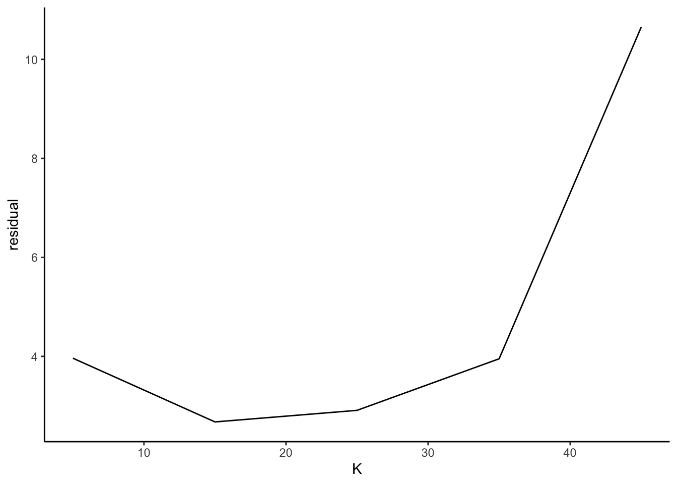
- It looks like K = 15 topics marginally has the lowest residuals, so we’ll go with that model.
Next, I pull out the values for beta (probability a word comes from a topic) and gamma (probability of a topic within a ‘document;’ here, the document is a song).
topic_model <- stms %>%
  filter(K == 15) %>%
  pull(topic_model) %>%
  .[[1]]

beta_tidy <- tidy(topic_model)

gamma_tidy <- tidy(topic_model, matrix = "gamma",
                 document_names = rownames(lyrics_dfm_en))
Here’s the real fun part — interpreting the topics. As a reminder, we are only analyzing the text of the lyrics (for now). We’ll get into audio features later in the visualizations.
I love pop music, but pop lyrics don’t tend to vary much. Nevertheless, I tried my best to label these topics for this heuristic exercise. I took liberty “labeling” the topics from the STMs into meaningful language. There are quantitative ways to do label topics, like with the labelTopics() function, which I also used to determine my labels. For instance, ‘rain’ and ‘loyalty’ were two of the top words for Topic 6 (labeled ‘longing’) in terms of highest probability and FREX. In Topic 8 (labeled ‘big dreams’), the top words for FREX and Score were ‘stamina,’ ‘dna,’ and ‘greatest.’
library(tidyr)

topic <- paste0("Topic ", unique(gamma_tidy$topic))
label <- c("party", "confident", "wanderer", "winning", "feeling free", "longing", "airy", "big dreams", "self-love", "friends", "mischievious", "nostalgic", "breaking out", "glow up", "in my feelings")
topic_label <- as.data.frame(cbind(topic, label))

songs <- c("Blue World", "2 Da Moon", "LOYALTY.", "7 rings", "About Today", "Don’t Call Me Up") # we'll dive into these songs later

gamma_abr <- gamma_tidy %>%
  mutate(topic = as.character(paste0("Topic ", topic)),
         topic = reorder(topic, gamma)) %>%
  separate(document, c("song", "artist", "row"), sep = "_", remove = FALSE) %>%
  filter(song %in% songs) %>%
  distinct(song, topic, gamma) %>%
  inner_join(topic_label, by = "topic")
We’ll also average the topic probability across all songs each year to see how my top lyrics’ topics change throughout time.
gamma_year <- gamma_tidy %>%
  mutate(topic = paste0("Topic ", topic),
         topic = reorder(topic, gamma)) %>%
  separate(document, c("song", "artist", "row"), sep = "_", remove = FALSE) %>%
  inner_join(tracks_full, by = "row") %>%
  mutate(artist = artist.x) %>%
  select(-artist.x, -artist.y) %>%
  inner_join(topic_label, by = "topic") %>%
  group_by(year, topic, label) %>%
  summarize(mean_gamma_yr = mean(gamma)) %>%
  ungroup() %>%
  mutate(year = as.numeric(as.character(year)))

hl_topics <- c("glow up", "wanderer", "in my feelings")
gr_topics <- c("party", "confident", "friends", "wanderer", "good times", "feeling free", "longing", "ethereal", "dreaming", "authentically me", "mischievious", "nostalgia", "breaking out", "in my feelings")

'%!in%' <- function(x,y)!('%in%'(x,y))

gamma_year <- gamma_year %>%
  mutate(high = case_when(
    label %in% c("glow up") ~ "A",
    label %in% c("wanderer") ~ "B",
    label %in% c("in my feelings") ~"C",
    label %in% gr_topics ~ "D"
  ))
Visualizing the data
Music as Tree Rings
We have a lot of data with this project, so I’ll start by looking at the basics. Let’s see who I listened to from 2014-2020 with this bubble chart resembling the cross-section of a tree:
library(ggiraph)
library(ggplot2)
library(packcircles)

top_artist <- tracks_full %>%
  group_by(artist, year) %>%
  summarise(count = n()) %>%
  arrange(-count) %>%
  arrange(year) %>%
  mutate(year = as.character(year))

packing <- circleProgressiveLayout(top_artist$count)

dat.gg <- circleLayoutVertices(packing)

colors1 <- as.character(c("#99B898", "#A8E6CE", "#FECEAB", "#FF847C", "#E84A5F", "#D7BDE2" , "#BEC0ED"))
year <- as.character(2014:2020)
colors_year <- as.data.frame(cbind(colors1, year))

top_artist <- top_artist %>%
  inner_join(colors_year) %>%
  mutate(colors = as.character(colors1))

top_artist$text <- paste(top_artist$artist, "\n", "Song count:", top_artist$count, "\n", "Year:", top_artist$year)

top_artist$id <- c(1:length(top_artist$artist))

dat.gg <- dat.gg %>%
  inner_join(top_artist, by = "id")

bubbles <- ggplot() +
  geom_polygon_interactive(data = dat.gg, aes(x, y, group = id, fill = factor(id), tooltip = top_artist$text[id], data_id = year), alpha = 0.6, show.legend = FALSE) +
  scale_fill_manual(values = top_artist$colors, labels = c('2014', '2015', '2016', '2017', '2018', '2019', '2020')) +
  theme_void() +
  guides(fill = guide_legend_interactive()) +
  # labs(title = "Annual rings of my artists' top songs") +
  theme(plot.margin=unit(c(0,0,0,0), "cm"),
        plot.title = element_text(size = 18, hjust = 0.5)) +
  coord_equal()

bubbles_interactive <- ggiraph(ggobj = bubbles, width_svg = 6.2, height_svg = 4.5)
bubbles_interactive There are more larger bubbles in recent years than earlier in my Spotify tenure. I must be listening to more songs by the same artists in 2018-2020.
My Music Moods
Next, I’ll use the audio features Spotify already provides when you collect data from their API. A common analysis among the spotifyr posts is to visualize the “mood” of a group of songs with Spotify’s audio features, not solely the lyrics like in the structural topic models. The “mood” can be understood by the valence (positivity rating where lower values are more “negative”) and energy (lower values have lower energy). If we make a plot of energy x valence like here in the Sentify Shiny app, we can see how my top songs fall into each quadrant.
This plotly graph shows the moods of my Top 100 songs throughout seven years of my Spotify Wrapped playlists. Click play or drag the the year bar to see how many songs are happy, pleasant, sad, or angry in each year.
library(plotly)
library(htmltools)

mood <- tracks_full %>%
  plot_ly(x = ~valence, y = ~energy, size = ~rank_weight, sizes = c(1, 350), text = ~artist, hoverinfo = "text")

mood2 <- mood %>%
  add_markers(color = ~year, showlegend = F, alpha = 0.05, alpha_stroke = 0.05, colors = colors1) %>%
  add_markers(color = ~year, frame = ~year, ids = ~artist, colors = colors1) %>%
  add_segments(x = 0.5, xend = 0.5, y = 0, yend = 1, showlegend = F, line = list(color = "#A9A9A9", width = 0.8)) %>%
  add_segments(x = 0, xend = 1, y = 0.5, yend = 0.5, showlegend = F, line = list(color = "#A9A9A9", width = 0.8)) %>%
  layout(xaxis = list(title = "Valence", showgrid = F, font = list(size = 18)),
         yaxis = list(title = "Energy", font = list(size = 18)),
         annotations = list(
           x = c(.05, .05, .95, .95),
           y = c(.05, .95, .05, .95),
           text = c("Sad", "Angry", "Pleasant", "Happy"),
           showarrow = FALSE,
           xanchor = "center",
           font = list(size = 15, color = "#547980")
         ),
         width = 600, height = 500
  ) %>%
  animation_opts(1000, easing = "elastic", redraw = FALSE) %>%
  animation_button(
    x = 1, xanchor = "right", y = 0, yanchor = "bottom"
  ) %>%
  animation_slider(
    currentvalue = list(prefix = "Year ", font = list(color = "#696969"))
  )

htmltools::div(mood2, align = "center")
Bubbles are songs. Bubble size corresponds to the song’s rank in the Top 100 (bigger points ranked more highly).
I seem to listen to more energetic songs as time goes on! 2014 seemed to be the “saddest” year based on the number of dots in that quadrant. Well, it was the end of my teenage years. I also had a lot of high energy songs in 2020, probably to counteract the perpetual quarantine.
Some Key Songs’ Topics
Now, let’s go back to the output from the structural topic model we ran in the Modeling the data section. Here are the gamma values (probabilities of a topic within a song) for a handful of songs that I picked out of arbitrary interest. This visualization is just to show the variability in evenness of gammas across songs.
group_colors1 <- c(`glow up` = "#B6B4C2",
                  wanderer = "#547980",
                  `in my feelings` = "#F9CDAD",
                  `breaking out` = "#AAC9CE",
                  confident = "#A8E6CE",
                  `big dreams` = "#CD7672",
                  `airy` = "#DCEDC2",
                  `feeling free` = "#63BCC9",
                  friends = "#E7E7E7",
                  `winning` = "#7E9680",
                  longing = "#ECD59F",
                  mischievious = "#8AB2E5",
                  nostalgic = "#FFDD94",
                  party = "#FF8C94",
                  `self-love` = "#E5C1CD")

ggplot(gamma_abr, aes(x = song, y = gamma, fill = label)) +
  geom_bar(stat = "identity", position = "stack") +
  scale_fill_manual(values = group_colors1) +
  labs(y = "Gamma values by song") +
  coord_flip() +
  theme_classic() +
  theme(legend.title = element_blank(),
        axis.title.y = element_blank(),
        text = element_text(size=12))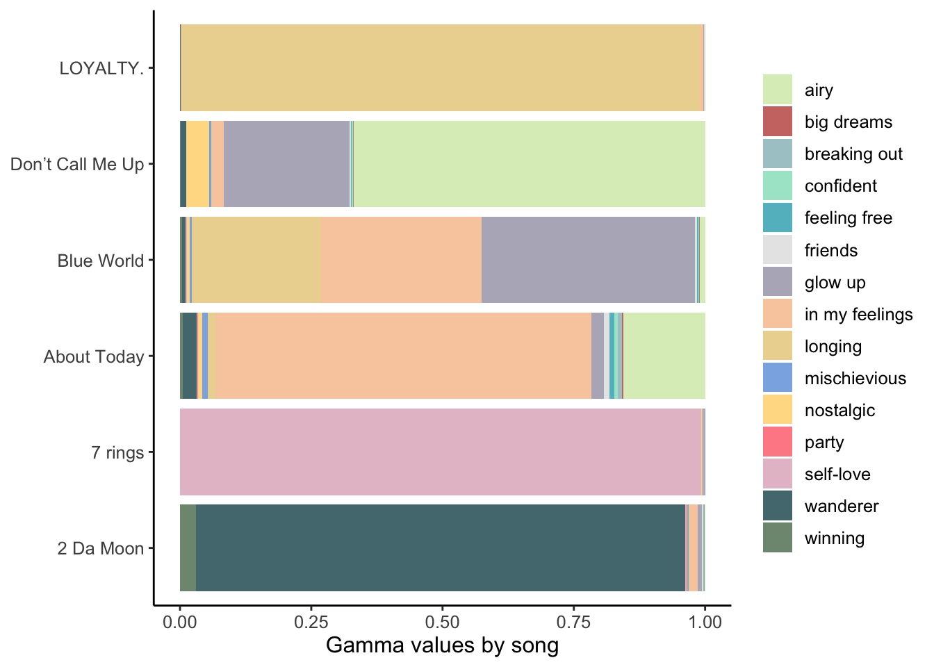
Lyrics’ Topics Over the Years
Finally, we’ll plot the mean gamma values by year. I’ve highlighted three topics (in color) to help tell the story of my Spotify Wrapped: ‘wanderer,’ ‘in my feelings,’ and ‘glow up.’
library(gganimate)

group_colors2 <- c(A = "#6C5B7B", B = "#547980", C = "#F9CDAD", D = "#D3D3D3")
group_alpha <- c(A = 1, B = 1, C = 1, D = 0.48)
group_size <- c(A = 1.55, B = 1.55, C = 1.55, D = 1)

time <- ggplot(gamma_year, aes(year, mean_gamma_yr, group = label, color = high, alpha = high, size = high)) +
  geom_line() +
  geom_segment(aes(xend = 2020.8, yend = mean_gamma_yr), linetype = 2) +
  geom_point(size = 2) +
  geom_text(aes(x = 2021, label = label), hjust = 0, size = 5.2) +
  scale_color_manual(values = group_colors2) +
  scale_alpha_manual(values = group_alpha) +
  scale_size_manual(values = group_size) +
  xlim(2014, 2021) +
  transition_reveal(year) +
  coord_cartesian(clip = 'off') +
  labs(y = 'Mean gamma') +
  theme_classic() +
  theme(legend.position = 'none',
        axis.title.x = element_blank(),
        plot.margin = margin(5, 75, 1, 5),
        text = element_text(size=20))

anim_save("time.gif", time, duration = 9.5)
A few possible reasons for these patterns:
- in my feelings: I was generally getting less and less in my feelings until…..2020…..
- wanderer: I was traveling a lot looking for grad schools and visiting friends around 2017-2018 and didn’t really travel in 2020.
- glow up: I was becoming my best self until…..2020…..(joking!)
Conclusions
A few caveats:
- This dataset is far from comprehensive or complete. It’s based on whatever formula Spotify uses to determine our yearly “Top Songs.” It’s unclear if the formula is based on listen count and/or other metrics.
- The analysis here doesn’t account for covariates like the song’s rank in the Top 100.
- The labels here are pretty subjective, but there doesn’t seem to be a standard way of labeling the topics. So I got to have fun thinking about them!
- I couldn’t filter out all non-English words as ‘stop words.’ For example, “Remember Me” by Miguel featuring Natalia Lafourcade has ~40% lyrics in Spanish. In this and other multilingual songs, I didn’t filter out all non-English words. This limitation inevitably messed with the exclusivity of words in topics and topic fitting.
A main takeaway:
Even though it was fun working with these data and packages, this modeling and visualization approach is no replacement for listening and feeling the music we love! No single topic label or audio metric can encapsulate the songs’ entire mood and meaning. Nevertheless, I enjoyed learning how to run and visualize structural topic models with this exercise. I hope some of this blog inspires you to look at your own listening habits!
Drop a comment as an issue or DM me on Twitter (at)danbtweeter!